Integrated Science Model
for Assessment of Climate Change (ISAM)

Figure 1: Click image to enlarge

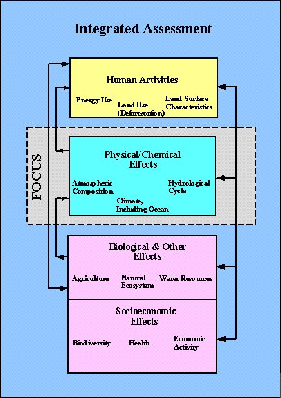
Thus, understanding of the relationships between human activities, potential changes to the Earth’s climate, and the resulting ecological and economic impacts and other effects on human welfare from these changes requires an interdisciplinary perspective involving the physical, biological, social and political sciences (Figure 1). In response to this need, a new paradigm has emerged - one whose main purpose is not only the acquisition of scientific knowledge, but the assimilation and communication of scientific results. Integrated Assessment Modeling (IAM) is a new important research methodology for examining the complex interactions among physical, and human systems. Rather than actually using many of the multi-dimensional and complicated expert models, IAM build on the knowledge achieved by each individual scientific discipline. The uses of such tools need to explicitly recognize and address the existence of considerable uncertainty and scientific debate surrounding climate issues. The model must be computationally efficient so that the many possibilities to be considered can be investigated on a personal computer or workstation in a matter of minutes, and must be simple and transparent, but based on solid science.

Figure 2: Click image to enlarge

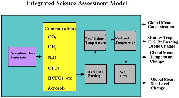
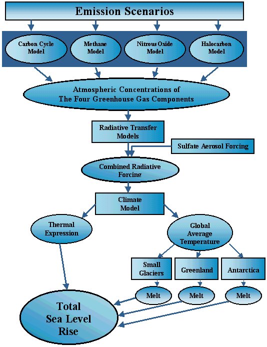
Our existing Integrated Science Assessment Model (ISAM) for assessment of climate change (Jain et al., 1994) consists of coupled modules for representation of the carbon cycle, effects of greenhouse gas emissions and aerosols on atmospheric composition, effects on global temperatures using an energy balance model, and processes affecting sea level change (Figure 2). This model has been used to estimate the relation between the time-dependent rate of greenhouse gas emissions and quantitative features of climate global temperature, the rate of temperature change, and sea level that are thought to be indicators of human impact on climate and ecosystems (Wigley et al., 1998). This model has also been applied to studies of Global Warming Potential (GWP, Wuebbles, et al., 1995), and the Economic-Damage Index (EDI, Hammitt et al., 1996) concepts.

Figure 3: Click image to enlarge

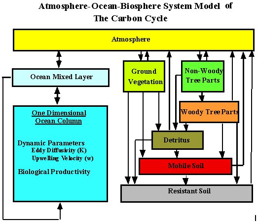
The concentration of CO₂ is calculated by a globally averaged carbon cycle model (Figure 3), which consists of four reservoirs, namely the atmosphere, the terrestrial biosphere, the mixed ocean layer, and the deep ocean (Jain et al., 1995, 1996). The atmosphere and the mixed layers are modeled as well mixed reservoirs. Transport of total inorganic carbon in the deep ocean is modeled by a partial differential equation, spanning time and ocean depth, which accounts for vertical diffusion and upwelling. The rate of transport in the deep ocean is dependent on two parameters: eddy diffusivity (k) and upwelling velocity (w). (Jain et al. 1995) determined parameter values k = 4700 m2/yr and w = 3.5 m/yr by calibration of model results to the estimated global-mean pre-anthropogenic depth-profile of ocean 14C concentration). Water upwells through the deep ocean column to the surface ocean layer from where it is returned, through a polar sea, to the bottom of the ocean column thereby completing the thermohaline circulation. Air-sea exchange is modeled by an air sea exchange coefficient in combination with the buffer factor that summarizes the chemical re-equilibration of sea water with respect to CO₂ variations. The buffer factor is calculated from the set of equations for borate, silicate, phosphate, and carbonate equilibrium chemistry and the temperature-dependent equilibrium constants. An additional source term is added to the model deep ocean to account for the oxidation of organic debris containing carbon removed in the surface ocean layer by photosynthesis and brought to the deep ocean by particulate settling.

To estimate the flux of CO₂ between the terrestrial biosphere and the atmosphere, a 6 box, globally-aggregated, terrestrial-biosphere sub-model is coupled to the atmosphere box. The six boxes represent ground vegetation, non-woody tree parts, woody tree parts, detritus, mobile soil (turn-over time 75 years), resistant soil (turnover time 500 years). The mass of the carbon contained in the different terrestrial reservoirs and the rate of exchange between them have been based on the analysis by Kheshgi et al. (1996). The photosynthetic rate of carbon fixation is modeled to increase logarithmically with atmospheric CO₂ concentration and is proportional to a CO₂ fertilization factor. The rate of photosynthesis by terrestrial biota is thought to be stimulated by increasing atmospheric carbon dioxide concentration. The increase in the rate of photosynthesis, relative to preindustrial times, is modeled to be proportional to the logarithm of the relative increase in atmospheric CO₂ concentration from its pre-industrial value of 278 ppm. The proportionality constant b, known as the CO₂ fertilization factor, is chosen to be 0.42. The rate coefficients for exchange to and from terrestrial biosphere boxes are temperature dependent according to an Arrhenius law.

Figure 4: Click image to enlarge

This model does contain temperature feedbacks on carbon cycle through the prescription of the temperature-dependent buffer factor, and exchange (respiration and photosynthesis) rates to and from the biosphere boxes which follow the "Q10 formulation" described in Kheshgi et al. (1996).

The existing carbon cycle model in ISAM was originally developed as a tool to predict the likely future changes of the atmospheric abundance of CO₂ dependent on the use of fossil fuels, deforestation and expansion of agriculture land. This schematic model for the carbon cycle is constructed to be consistent with current understanding of the global carbon cycle. Testing of the capability of the model to represent this understanding has, in part, been based on the analysis of tracer records such as those for 13C and 14C (Figure 4). For the last two IPCC assessments, our carbon cycle model has also been used to assess the future scenarios (Schimel et al., 1995, 1996, 1997).

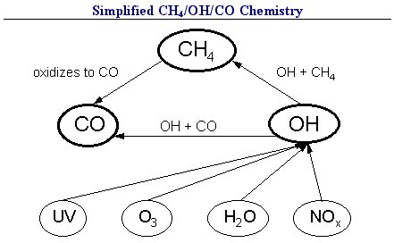
The methane concentration in the atmosphere is calculated by simulating the main atmospheric chemical processes influencing the global concentrations of CH₄, CO, and OH, using the global CH₄-CO-OH cycle module (Figure 5). The removal rates of CH₄ and CO are determined by accounting for the uptake by soils, transport to the stratosphere, and oxidation by OH radicals. We assume the uptake velocity by soils and the transport velocity to the stratosphere to be time-independent, although there is evidence that these values change with time.

Figure 5: Click image to enlarge

Reaction with the OH radical is responsible for up to 90% of the tropospheric CH₄ sink, making the tropospheric concentrations of OH and CH₄ the most important factors influencing the rate at which CH₄ is destroyed. OH concentration is primarily determined by the concentrations of CH₄, CO, NOx, non-methane hydrocarbons (NMHCs), tropospheric ozone, and water vapor. With sharp spatial and temporal gradients, an observation-based estimate of the global concentration of OH is difficult to make, as are the rates of OH production and destruction which depend non-linearly on other atmospheric constituents. In attempts to adequately represent all significant chemical and dynamic processes determining local OH concentrations, detailed two- or three-dimensional chemical transport models of the atmosphere have been used. However, to incorporate OH chemistry into methane modeling for scenario analysis, simplified schemes are used which reproduce the important influences on OH while remaining straightforward and computationally feasible. In ISAM, the concentration of OH is determined by the photochemical balance between the total tropospheric production of OH and the loss rate due to reaction with CH₄, CO and NMHCs [Jain et al., 1994]. The loss rate of OH is determined by reactions between OH and CH₄, CO and NMHCs with reaction rates. The production rate of OH is based on a correlation giving global OH production rate as a function of NOx emissions and CH₄ concentration based on results of a well established 2-D (latitude and altitude) chemical-radiative transport model of the global atmosphere (Wuebbles et al., 1991, 1998). The 2-D model used has a full representation of NOx, HOx, CH₄, O₃, and CO chemistry relevant to tropospheric and stratospheric chemistry. The OH production rate correlation used in ISAM was derived from the following results of this 2-D model: a 110-year simulation of the Intergovernmental Panel on Climate Change (IPCC) scenario IS92a and perturbations from 1990 atmospheric conditions.

Figure 6: Click image to enlarge

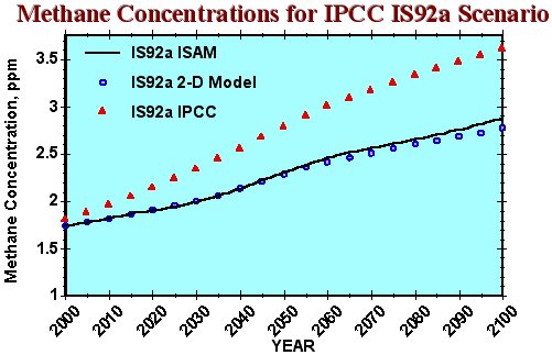
In Figure 6 the ISAM CH₄ concentration results for the IPCC IS92a scenario are compared with those of the 2-D model. Input to the 2-D model are zonal patterns of 1990 CH₄, NOx, CO and NMHC emissions which are scaled by global emission rates which grow according to the IS92a scenario. The ISAM model reproduces the globally averaged 2-D model result up until 2060, after which the ISAM CH₄ concentration is slightly higher; the close reproduction is not surprising since OH production from the 2-D model result was used to calibrate OH production in ISAM. However, this analysis of the IS92a scenario gives a CH₄ concentration which is about 20% lower than the IPCC (1995) projection of 3.6 ppmv in 2100, which prescribed constant NOx , CO and NMHC emissions at 1990 rates.

FIGURES
Figure 1 | Figure 2 | Figure 3 | Figure 4 | Figure 5 | Figure 6